Mesh adaption

In this section, we propose to illustrate on a 2d example the various tools available in Muscat for mesh adaption.

Modeling the problem

Consider the pierced plate shown in the following figure (length 4 m, width 2m):

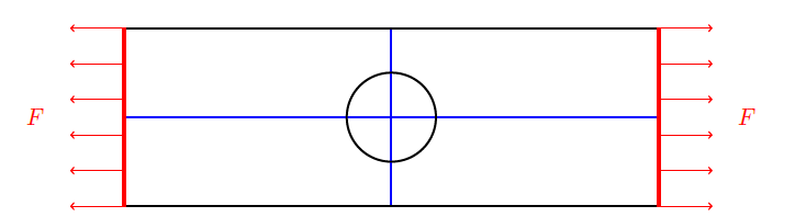
We want to calculate the plate deformation when it is subjected to a tension of F = 1 GPa at both ends, as depicted in the figure. The plate is assumed to be made of a homogeneous, isotropic linear elastic material with Poisson ratio ν = 0.3 and Young modulus E = 10 GPa. By virtue of symmetry, we can solve the problem on any quarter of the plate, imposing zero transverse displacements along the symmetry axes, shown in blue.

Numerical solution using Muscat

Muscat’s integrated finite element solver is used to solve the problem.

First we initialize a new variational problem.

import numpy as np

from Muscat.FE.UnstructuredFeaSym import UnstructuredFeaSym

problem = UnstructuredFeaSym(spaceDim=2)

Then we choose a linear elastic formulation with isoparametric finite elements

from Muscat.FE.SymPhysics import MechPhysics
mechPhysics = MechPhysics(dim=2)
mechPhysics.planeStress = True
mechPhysics.SetSpaceToLagrange(isoParam=True)

and we define the material properties and the loading.

mechPhysics.AddBFormulation("bulkA", mechPhysics.GetBulkFormulation(10., 0.3))
mechPhysics.AddBFormulation("2D", mechPhysics.GetBulkFormulation(10., 0.3))
mechPhysics.AddLFormulation("Y1", mechPhysics.GetPressureFormulation(1))

problem.physics.append(mechPhysics)

We impose the Dirichlet boundary conditions.

from Muscat.FE.KR.KRBlock import KRBlockVector

dirichlet_lock_x = KRBlockVector().AddArg("u").On('x0').On('X0').BlockDirection0()
problem.solver.constraints.AddConstraint(dirichlet_lock_x)

dirichlet_lock_y = KRBlockVector().AddArg("u").On('y0').BlockDirection1()
problem.solver.constraints.AddConstraint(dirichlet_lock_y)

We read the mesh and link it to the problem.

from Muscat.IO.XdmfReader import ReadXdmf
from Muscat.TestData import GetTestDataPath

mesh = ReadXdmf(GetTestDataPath()+"holeplatequad.xdmf")

print("Initial", mesh)

problem.SetMesh(mesh)
problem.ComputeDofNumbering()

Initial Mesh
  Number Of Nodes    : 1123
    Tags : (x0y0:1) (x1y0:1) (x0y1:1) (x1y1:1)
  Number Of Elements : 492
    ElementsContainer,   Type : (ElementType.Bar_3,70),   Tags : (X1:20) (Y0:10) (Skin:60) (X0:20) (y0:5) (x0:5) (Y1:10)
    ElementsContainer,   Type : (ElementType.Quadrangle_8,200),   Tags : (2D:200)
    ElementsContainer,   Type : (ElementType.Triangle_6,222),   Tags : (bulkA:222)

Finally we solve the variational formulation

k,f = problem.GetLinearProblem()
problem.ComputeConstraintsEquations()
problem.Solve(k,f)
problem.PushSolutionVectorToUnknownFields()

from Muscat.FE.Fields.FieldTools import GetPointRepresentation

sol = GetPointRepresentation(problem.unknownFields)
mesh.nodeFields["solution"] = sol

and plot the solution.

import pyvista as pv
pv.global_theme._jupyter_backend = 'panel' # remove this line to get interactive 3D plots
from Muscat.Bridges.PyVistaBridge import MeshToPyVista

pyVistaMesh = MeshToPyVista(mesh)
edges = pyVistaMesh.separate_cells().extract_feature_edges()
pl = pv.Plotter()
pl.add_mesh(pyVistaMesh, scalars="solution", scalar_bar_args=dict(vertical=True))
pl.add_mesh(edges, color="black")
pl.show(cpos= "xy")

Mesh adaption

Linear simplex meshes

There is no reliable remesher for meshes other than linear simplex meshes, i.e. those composed of points, 2-point bars, 3-point triangles and 4-point tetrahedrons. Muscat offers tools for transforming any mesh (with pyramids, prisms, quads, hexa, etc.) into a simplex mesh, while guaranteeing the transfer of tags and associated fields.

First we can linearize the mesh:

from Muscat.MeshTools.MeshTetrahedrization import FromQuadToLinear

mesh = FromQuadToLinear(mesh)

print("Linear", mesh)

Linear Mesh
  Number Of Nodes    : 351
    Tags : (x0y0:1) (x1y0:1) (x0y1:1) (x1y1:1)
  Number Of Elements : 492
    ElementsContainer,   Type : (ElementType.Bar_2,70),   Tags : (y0:5) (Y0:10) (X1:20) (Y1:10) (X0:20) (x0:5) (Skin:60)
    ElementsContainer,   Type : (ElementType.Quadrangle_4,200),   Tags : (2D:200)
    ElementsContainer,   Type : (ElementType.Triangle_3,222),   Tags : (bulkA:222)
  nodeFields         : ['solution']

Then we can convert it to a simplex mesh:

from Muscat.MeshTools.MeshTetrahedrization import Tetrahedrization

mesh = Tetrahedrization(mesh)

print("Linear simplex", mesh)

Linear simplex Mesh
  Number Of Nodes    : 351
    Tags : (x0y0:1) (x1y0:1) (x0y1:1) (x1y1:1)
  Number Of Elements : 692
    ElementsContainer,   Type : (ElementType.Bar_2,70),   Tags : (y0:5) (Y0:10) (X1:20) (Y1:10) (X0:20) (Skin:60) (x0:5)
    ElementsContainer,   Type : (ElementType.Triangle_3,622),   Tags : (bulkA:222) (2D:400)
  nodeFields         : ['solution']

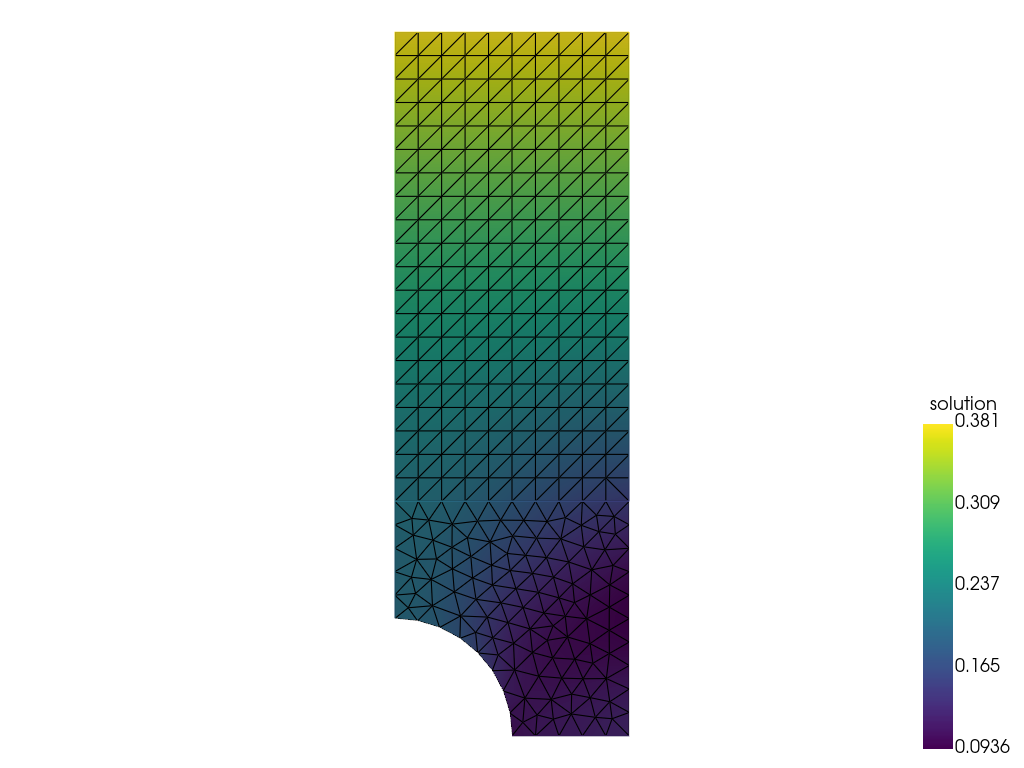
And plot the resulting mesh with the solution.

pyVistaMesh = MeshToPyVista(mesh)
pl = pv.Plotter()
pl.add_mesh(pyVistaMesh, scalars="solution", show_edges=True, scalar_bar_args=dict(vertical=True))
pl.show(cpos= "xy")

Remeshing from a mesh size map

The first step is to select a criterion on which to adapt the mesh. This criterion can be any scalar field defined at mesh nodes. Here, for example, we will choose the displacement norm, and we want to obtain a mesh which guarantees that the relative error committed on this quantity of interest is lower than 1e-5 at all points.

psi = np.linalg.norm(mesh.nodeFields["solution"], axis=1)
err = 1e-5

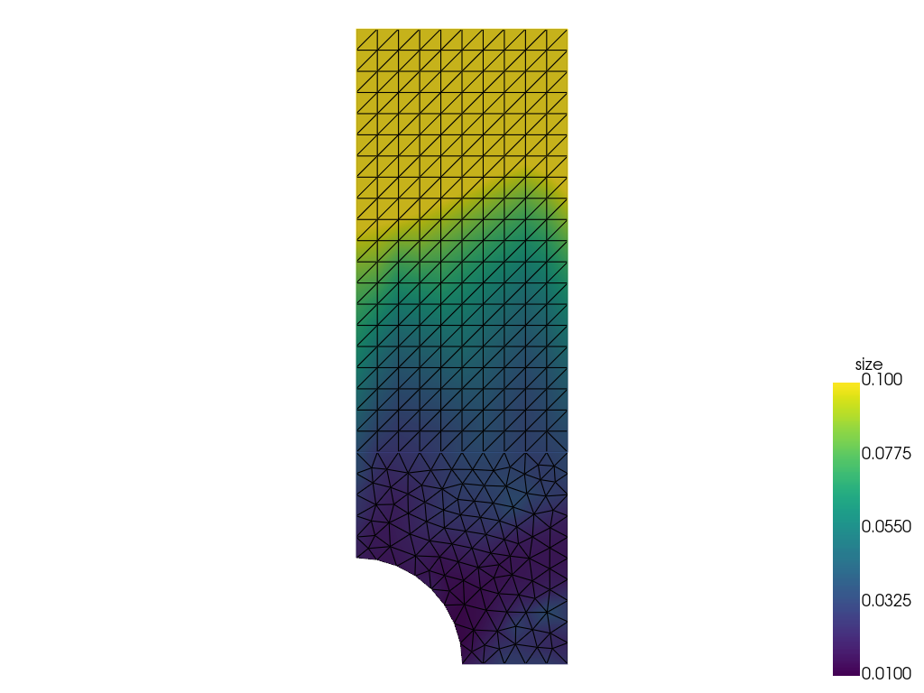
The second step is to compute thank to Muscat the ideal mesh size associated with this criterion.

from Muscat.MeshTools.AnisotropicMetricComputation import ComputeMetric

siz = ComputeMetric(mesh, psi, err=err, isotropic=True)

mesh.nodeFields["size"] = siz

pyVistaMesh = MeshToPyVista(mesh)
pl = pv.Plotter()
pl.add_mesh(pyVistaMesh, scalars="size", show_edges=True, scalar_bar_args=dict(vertical=True), clim=[0.01, 0.1])
pl.show(cpos= "xy")

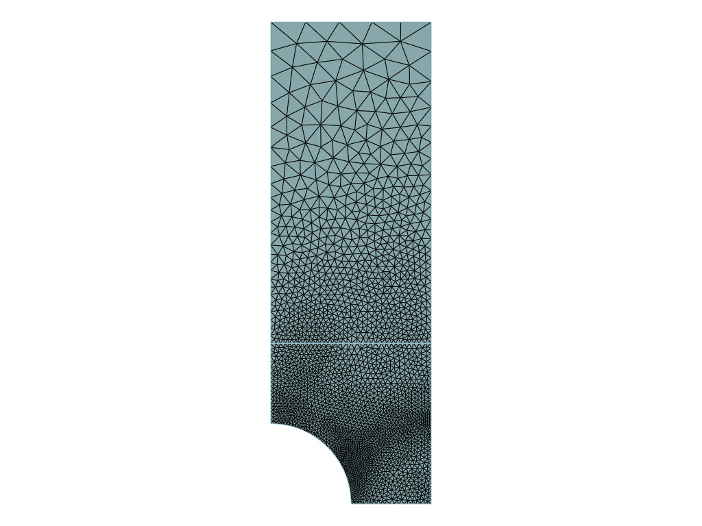
The last step consists in using a remesher to build the desired mesh from the mesh size map.

from Muscat.MeshTools.Remesh import Remesh

iso_mesh = Remesh(mesh, metric=siz)

print("Isotropic", iso_mesh)

pyVistaMesh = MeshToPyVista(iso_mesh)
pl = pv.Plotter()
pl.add_mesh(pyVistaMesh, show_edges=True)
pl.show(cpos= "xy")

Isotropic Mesh
  Number Of Nodes    : 2682
    Tags : (Corners:5) (Required:5) (x1y1:1) (x0y1:1) (x1y0:1) (x0y0:1)
  Number Of Elements : 5396
    ElementsContainer,   Type : (ElementType.Bar_2,218),   Tags : (Ridges:184) (x0:17) (X0:24) (Skin:88) (Y1:5) (X1:25) (Y0:34) (y0:20)
    ElementsContainer,   Type : (ElementType.Triangle_3,5178),   Tags : (2D:1394) (bulkA:3784)

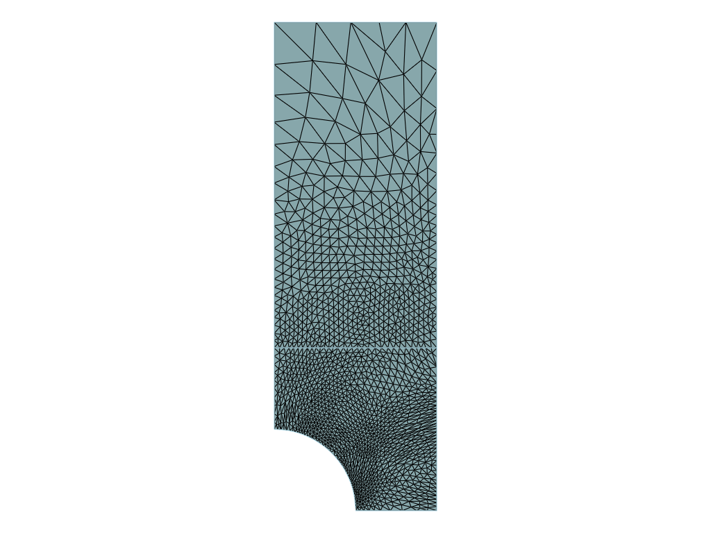
Remeshing from a metric computation

From the same criterion, it is also possible to compute an anisotropic metric, that gives at each node the principal directions and the associated ideal mesh sizes.

met = ComputeMetric(mesh, psi, err=err)

The remesher will then produce an anisotropic mesh.

aniso_mesh = Remesh(mesh, metric=met)

print("Anisotropic", aniso_mesh)

pyVistaMesh = MeshToPyVista(aniso_mesh)
pl = pv.Plotter()
pl.add_mesh(pyVistaMesh, show_edges=True)
pl.show(cpos= "xy")

Anisotropic Mesh
  Number Of Nodes    : 1607
    Tags : (Corners:5) (Required:5) (x1y1:1) (x0y1:1) (x1y0:1) (x0y0:1)
  Number Of Elements : 3244
    ElementsContainer,   Type : (ElementType.Bar_2,184),   Tags : (Ridges:152) (x0:10) (X0:23) (Skin:84) (Y1:5) (X1:24) (Y0:32) (y0:10)
    ElementsContainer,   Type : (ElementType.Triangle_3,3060),   Tags : (2D:1064) (bulkA:1996)

Intersection of metrics

In Muscat, it is possible to remesh with respect to several criteria simultaneously. In the following example, we request a mesh that is not only optimal with respect to the previously calculated solution, but also with the analytical function |y - x - 2|.

We first compute the metric associated with the analytical function.

psi2 = np.abs(mesh.nodes[:, 1]-mesh.nodes[:, 0]-2)
met2 = ComputeMetric(mesh, psi2, err=1e-4)

And we intersect it with the previous metric.

from Muscat.MeshTools.AnisotropicMetricComputation import IntersectionOfMetrics

met3 = IntersectionOfMetrics(metrics=[met, met2])

/home/docs/checkouts/readthedocs.org/user_builds/muscat/conda/2.5.1.1/lib/python3.11/site-packages/cvxpy/problems/problem.py:1539: UserWarning: Solution may be inaccurate. Try another solver, adjusting the solver settings, or solve with verbose=True for more information.
  warnings.warn(

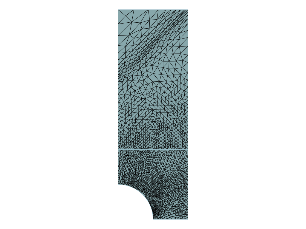
We can use this new metric to obtain a mesh that is adapted to both criteria.

newMesh = Remesh(mesh, metric=met3)

print("Intersected", newMesh)

pyVistaMesh = MeshToPyVista(newMesh)
pl = pv.Plotter()
pl.add_mesh(pyVistaMesh, show_edges=True)
pl.show(cpos="xy")

Intersected Mesh
  Number Of Nodes    : 1705
    Tags : (Corners:5) (Required:5) (x1y1:1) (x0y1:1) (x1y0:1) (x0y0:1)
  Number Of Elements : 3440
    ElementsContainer,   Type : (ElementType.Bar_2,200),   Tags : (Ridges:168) (x0:10) (X0:30) (Skin:101) (Y1:10) (X1:29) (Y0:32) (y0:10)
    ElementsContainer,   Type : (ElementType.Triangle_3,3240),   Tags : (2D:1253) (bulkA:1987)