Computation of strains using Muscat Integrator

The goal of this tutorial is to show how one can use the integrator to compute all sorts of physical quantities in meshes either on elements or nodes

Problem definition

Let us consider a \(10\times10\times10\) cube on which we know the nodal displacements but not the strains

from Muscat.MeshTools.ConstantRectilinearMeshTools import CreateConstantRectilinearMesh
from Muscat.MeshTools.MeshTetrahedrization import Tetrahedrization

## Create the cube mesh
mesh = Tetrahedrization(CreateConstantRectilinearMesh([10,10,10],[0.,0.,0.],[1/9,1/9,1/9]))

## Create fake displacement fields that have a non constant gradient (and thus strain)
mesh.nodeFields["U_0"]=(mesh.nodes[:,0]**2).copy(order='C')
mesh.nodeFields["U_1"]=(mesh.nodes[:,1]**2).copy(order='C')
mesh.nodeFields["U_2"]=(mesh.nodes[:,2]**2).copy(order='C')
print(mesh)

OMP: Warning #42: OMP_PROC_BIND: ""spread"" is an invalid value; ignored.
OMP: Warning #250: OMP_PLACES: syntax error, using cores.

Mesh
  Number Of Nodes    : 1000
    Tags :
  Number Of Elements : 4374
    ElementsContainer,   Type : (ElementType.Tetrahedron_4,4374),   Tags :
  nodeFields         : ['U_0', 'U_1', 'U_2']

The displacements are continuous, piecewise linear (P1 elements) of dimension 3, thus the strain is a symetric tensor constant per element (P0 field) that is in dimension 6 (in Voigt notation)

import Muscat.FE.SymWeakForm as wf
from Muscat.FE.DofNumbering import ComputeDofNumbering
from Muscat.FE.Spaces.FESpaces import LagrangeSpaceGeo,LagrangeSpaceP0

## Defining fields
StrainField = wf.GetField("Strain", 6, 3)
StrainFieldTest = wf.GetTestField("Strain", 6, 3)
RealDisplacements = wf.GetField("RealDisplacements", 3, 3)

## Defining numbering for each of the spaces
numbering_center = ComputeDofNumbering(mesh, LagrangeSpaceP0)
numbering = ComputeDofNumbering(mesh, LagrangeSpaceGeo, fromConnectivity=True)

Now we are defining the weak form and the FEfields for the integral, the space and numbering are key to defining the support of the field. please note that the names of the FEFields are matching exactly the name of the fields defined above.

In order to evaluate the strain fields we define the following weak form:

\[\varepsilon(u):\varepsilon^*\]

Where \(\varepsilon\) is the strain tensor (i.e. the symetrized gradient) and \(u\) the displacement vector.

So as to avoid duplicate equations we resort to the Voigt notation that keeps only the symmetric part of the strain tensor:

\[\varepsilon_{\text{Voigt}}(u).\varepsilon_{\text{Voigt}}^*.\]

We provide the data for the displacements when defining the displacement FEFields. However for the Strain field we do not provide data: it is the unknown in our problem

from Muscat.FE.Fields.FEField import FEField
from Muscat.FE.SymWeakForm import Strain,ToVoigtEpsilon

## Weak form using only the Test field in order to compute a right hand side
wform =  ToVoigtEpsilon(Strain(RealDisplacements)).T*StrainFieldTest

## Displacement fields: defined on P1 space and with the associated numbering
## We provide the data using the data option
known_fields = [ FEField(name = f"RealDisplacements_{i}",
                    mesh = mesh,
                    space = LagrangeSpaceGeo ,
                    numbering = numbering,
                    data = mesh.nodeFields[f"U_{i}"],
                    ) for i in range(3)]

## Strain fields: defined on P0 space with the element numbering
## We provide no data here since this is the unknown fields
unknownFields = [FEField(name = f"Strain_{i}",
                            mesh = mesh,
                            space = LagrangeSpaceP0,
                            numbering = numbering_center
                            ) for i in range(6) ]

Now we want to get the value of the strains at the center of the elements thus we need to specify two things to the integrator:

• Compute the value only on the element center by setting the integration rule to elementCenterQuadrature

• We don’t actually want to perform an integration but rather an evaluation thus we need to set the argument onlyEvaluation to True: this skips the multiplication by the quadratures weights and the determinant of the jacobian of the current element

from Muscat.MeshContainers.Filters.FilterObjects import ElementFilter
from Muscat.FE.Integration import IntegrateGeneral
from Muscat.FE.IntegrationRules import elementCenterQuadrature

# We filter the elements of dimensionnality 3 however if we want to evaluate on skin elements (2D) the filter has to be updated accordingly
ff = ElementFilter(dimensionality = 3)
## Displacements are provided as known_field whether the strain as an unknown
## Quadrature is taken for evaluation at the center of the elements
## We set onlyEvaluation to True to deactivate the multiplication of weights and jacobian
m, f = IntegrateGeneral(mesh = mesh,
                            wform = wform,
                            constants = {},
                            fields = known_fields,
                            unknownFields = unknownFields,
                            integrationRule= elementCenterQuadrature,
                            onlyEvaluation= True,
                            elementFilter = ff)

## Reshaping the strains in the voigt notation (NElement,6)
strains = f.reshape(6,f.shape[0]//6).T

## Or using Muscat FieldTools functions for higher level of abstraction
from Muscat.FE.Fields.FieldTools import VectorToFEFieldsData, GetCellRepresentation
# from to linear algebra (f) to field data
VectorToFEFieldsData(f, unknownFields)
# from fields to cell data for visualization
strains = GetCellRepresentation(unknownFields, fillValue=0.0, method='mean')


## Assigning the element fields to the mesh
mesh.elemFields["e_xx"]=strains[:,0]
mesh.elemFields["e_yy"]=strains[:,1]
mesh.elemFields["e_zz"]=strains[:,2]
mesh.elemFields["e_yz"]=strains[:,3]
mesh.elemFields["e_xz"]=strains[:,4]
mesh.elemFields["e_xy"]=strains[:,5]

# Plotting the mesh
import pyvista as pv
pv.global_theme._jupyter_backend = 'panel'
from Muscat.Bridges.PyVistaBridge import MeshToPyVista

plotter = pv.Plotter()
camera = pv.Camera()

plotter.add_text("Strain xx component", font_size=10)
plotter.add_mesh(MeshToPyVista(mesh), scalars="e_xx", show_edges=True, show_scalar_bar=False, edge_color="grey", cmap="rainbow_r")
plotter.add_scalar_bar(title="Strain",vertical=True)
camera.position = (-0.635, 3.325, 1.887)
camera.focal_point = (0.5,0.5,0.5)
camera.up = (0.133,-0.393,0.909)
plotter.camera=camera
plotter.show()

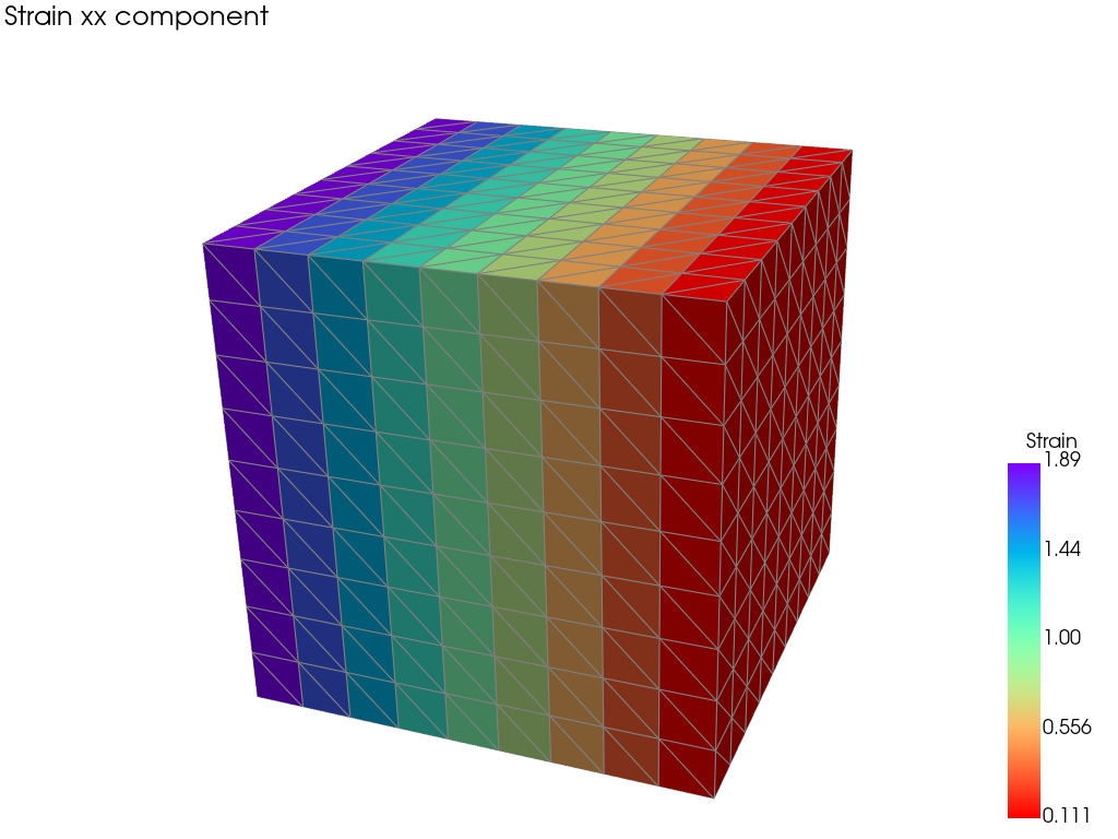
The strains are constant per element as expected

However for the sake of visualization we would like to interpolate these values from the nodes rather than displaying on elements therefore we will make the evaluation on the nodes rather than the center

Computing strains on nodes

Method 1: Using the element computation

One way to smooth the plot is to resort to the previous element computation and get the point representation

from Muscat.FE.Fields.FieldTools import GetPointRepresentation
# from fields to point data for visualization
strains_at_points = GetPointRepresentation(unknownFields, fillValue=0.0)

mesh.nodeFields["e_xx"]=strains_at_points[:,0]
mesh.nodeFields["e_yy"]=strains_at_points[:,1]
mesh.nodeFields["e_zz"]=strains_at_points[:,2]
mesh.nodeFields["e_yz"]=strains_at_points[:,3]
mesh.nodeFields["e_xz"]=strains_at_points[:,4]
mesh.nodeFields["e_xy"]=strains_at_points[:,5]
from Muscat.Bridges.PyVistaBridge import PlotMesh
PlotMesh(mesh, scalars="e_xx")

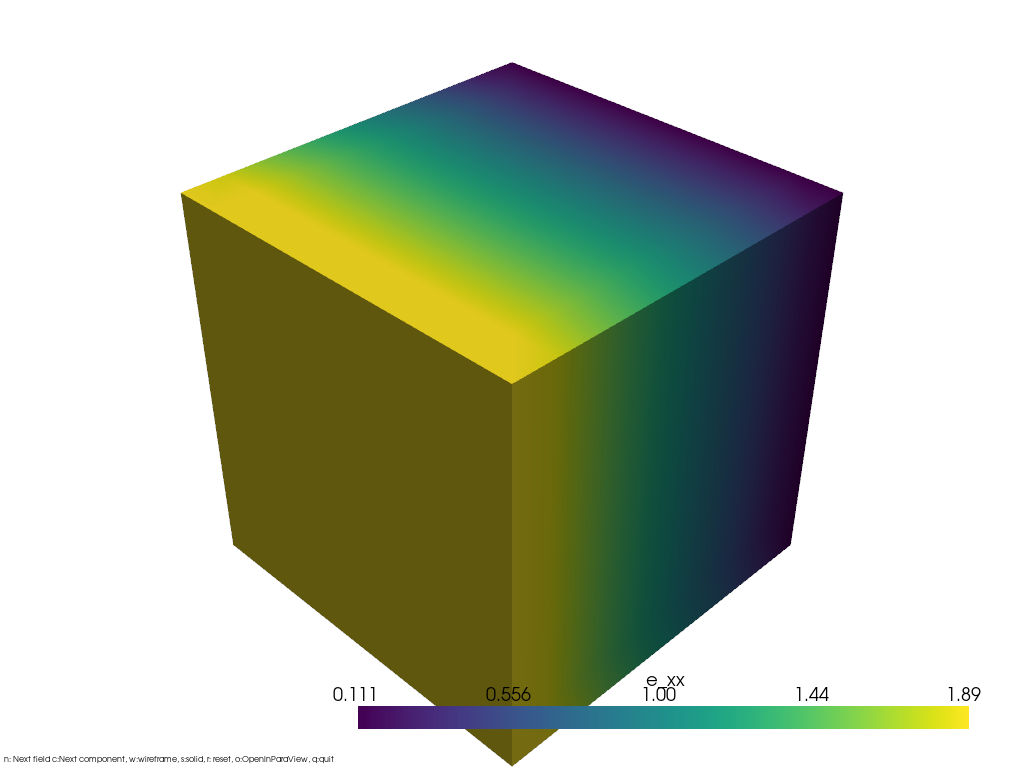
However we might not have the element representation or prefer using node evaluations in case we have higher order elements that don’t have a constant strain per element

Method 2: If the elementwise computation is not available

The code will be similar to the element-wise computation step however the strains will now be expressed as a P1 field the first part of the code (definition of the mesh + definition of the fields) does not change:

from Muscat.MeshTools.ConstantRectilinearMeshTools import CreateConstantRectilinearMesh
from Muscat.MeshTools.MeshTetrahedrization import Tetrahedrization

## Create the cube mesh
mesh = Tetrahedrization(CreateConstantRectilinearMesh([10,10,10],[0.,0.,0.],[1/9,1/9,1/9]))

## Create fake displacement fields that have a non constant gradient (and thus strain)
mesh.nodeFields["U_0"]=(mesh.nodes[:,0]**2).copy(order='C')
mesh.nodeFields["U_1"]=(mesh.nodes[:,1]**2).copy(order='C')
mesh.nodeFields["U_2"]=(mesh.nodes[:,2]**2).copy(order='C')
print(mesh)

import Muscat.FE.SymWeakForm as wf
from Muscat.FE.DofNumbering import ComputeDofNumbering
from Muscat.FE.Spaces.FESpaces import LagrangeSpaceGeo

## Defining fields
StrainField = wf.GetField("Strain", 6, 3)
StrainFieldTest = wf.GetTestField("Strain", 6, 3)
RealDisplacements = wf.GetField("RealDisplacements", 3, 3)

Mesh
  Number Of Nodes    : 1000
    Tags :
  Number Of Elements : 4374
    ElementsContainer,   Type : (ElementType.Tetrahedron_4,4374),   Tags :
  nodeFields         : ['U_0', 'U_1', 'U_2']

However we no longer need the numbering for the element center dofs

## Defining numbering for each of the spaces
## note here that we no longer use the P0 space
numbering = ComputeDofNumbering(mesh, LagrangeSpaceGeo, fromConnectivity=True)

The FEFields are now all expressed on the P1 FESpace:

from Muscat.FE.Fields.FEField import FEField
from Muscat.FE.SymWeakForm import Strain,ToVoigtEpsilon


## The weak form does not change
wform =  ToVoigtEpsilon(Strain(RealDisplacements)).T*StrainFieldTest
## Displacement fields: defined on P1 space and with the associated numbering
## We provide the data using the data option
known_fields = [ FEField(name = f"RealDisplacements_{i}",
                    mesh = mesh,
                    space = LagrangeSpaceGeo ,
                    numbering = numbering,
                    data = mesh.nodeFields[f"U_{i}"],
                    ) for i in range(3)]

## Strain fields: defined on P1 space with the same numbering than the Displacement fields
## We provide no data here since this is the unknown fields
unknownFields = [FEField(name = f"Strain_{i}",
                            mesh = mesh,
                            space = LagrangeSpaceGeo,
                            numbering = numbering
                            ) for i in range(6) ]

And we need to change the integrationRule to compute the values on the nodes rather than the element centers (using the NodalEvaluationP1Quadrature)

from Muscat.FE.IntegrationRules import NodalEvaluationP1Quadrature
from Muscat.MeshContainers.Filters.FilterObjects import ElementFilter
from Muscat.FE.Integration import IntegrateGeneral

ff = ElementFilter(dimensionality = 3)

## Displacements are provided as known_field whether the strain as an unknown
## Quadrature is taken for evaluation at the nodes
## We set onlyEvaluation to True
m, f = IntegrateGeneral(mesh = mesh,
                        wform = wform,
                        constants = {},
                        fields = known_fields,
                        unknownFields = unknownFields,
                        integrationRule= NodalEvaluationP1Quadrature,
                        onlyEvaluation= True,
                        elementFilter = ff)

## Either reshaping manually
strains = f.reshape(6,f.shape[0]//6).T

## Or using Muscat FieldTools functions for higher level of abstraction
from Muscat.FE.Fields.FieldTools import VectorToFEFieldsData, GetPointRepresentation
# from to linear algebra (f) to field data
VectorToFEFieldsData(f, unknownFields)
# from fields to point data for visualization
strains = GetPointRepresentation(unknownFields, fillValue=0.0)

However this results in the values of the nodes being summed in the f vector rather than averaged, therefore we need to perform an extra step for normalizing with respect to the number of times a node has been counted.

import numpy as np
counts = np.zeros(mesh.GetNumberOfNodes())
for selection in ff(mesh):
    conn = selection.elements.connectivity[selection.indices, :]

    np.add.at(counts,conn.ravel(),np.ones_like(conn.ravel()))
strains /=counts[:,None]

## now the strain field is a nodal one
mesh.nodeFields["e_xx"]=strains[:,0]
mesh.nodeFields["e_yy"]=strains[:,1]
mesh.nodeFields["e_zz"]=strains[:,2]
mesh.nodeFields["e_yz"]=strains[:,3]
mesh.nodeFields["e_xz"]=strains[:,4]
mesh.nodeFields["e_xy"]=strains[:,5]


# Plotting the mesh
import pyvista as pv
pv.global_theme._jupyter_backend = 'panel'
from Muscat.Bridges.PyVistaBridge import MeshToPyVista

plotter = pv.Plotter()
camera = pv.Camera()

plotter.add_text("Strain xx component", font_size=10)
plotter.add_mesh(MeshToPyVista(mesh), scalars="e_xx", show_edges=True, show_scalar_bar=False, edge_color="grey", cmap="rainbow_r")
plotter.add_scalar_bar(title="Strain",vertical=True)
camera.position = (-0.635, 3.325, 1.887)
camera.focal_point = (0.5,0.5,0.5)
camera.up = (0.133,-0.393,0.909)
plotter.camera=camera
plotter.show()

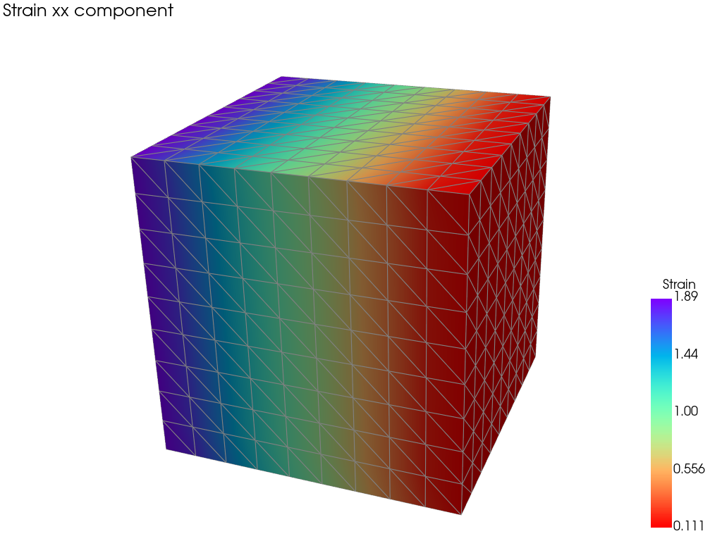
In the resulting mesh you have a P1 strain field much better looking

Although this image is much more suitable for visualizing it is no representative of the actual values of the strain that are accurately presented in the element-wise plot